How Are S&P 500 Returns Distributed Throughout the Year?
It is well known that the S&P 500, like US equity indexes more broadly, has a strong long-term bullish bias. What is less well understood is how this upward tendency is distributed throughout the year.
To explore this question, we can use Bias Finder, our proprietary analysis software, which allows us to examine the behavior of individual markets across different time horizons, including the full 365-day calendar year.
In this case, we want to determine whether E-mini S&P 500 futures (@ES) exhibit seasonal windows that are more profitable than others and, more importantly, whether these windows are connected in some way.
Figure 1 shows the average annual performance of E-mini S&P 500 futures. Three particularly significant periods are highlighted: the red box marks the seasonal window running from the beginning of the year through the end of June, the green box represents the second half of the year, from July through December, and the blue box covers the period from approximately the second week of October through year-end.
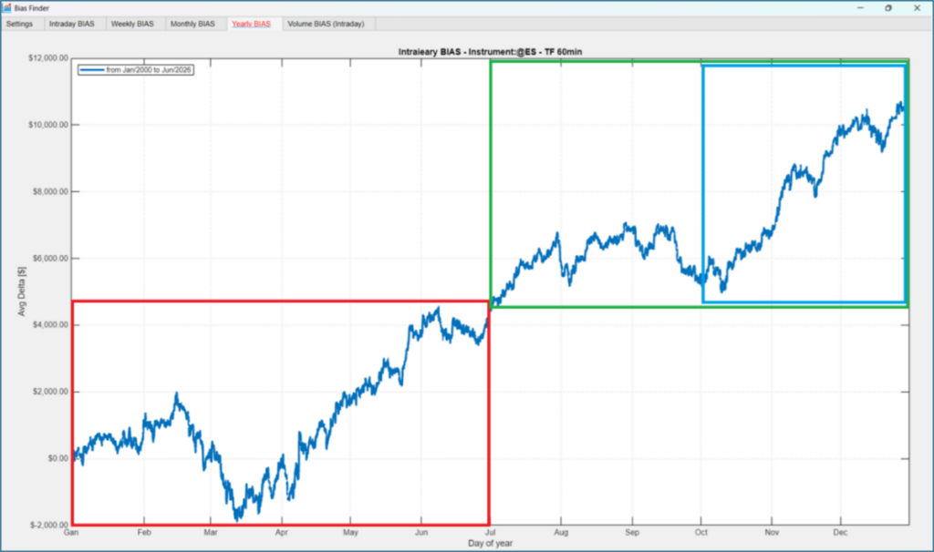
Figure 1 – Average annual performance of E-mini S&P 500 futures and the main seasonal windows analyzed.
At first glance, beyond the underlying bullish bias shared by all the periods analyzed, the second half of the year appears to be generally more bullish than the first, with particularly strong acceleration during the fourth quarter.
This raises an interesting question: could there be a relationship between these seasonal windows that might allow us to outperform a simple buy-and-hold approach? For example, if the market delivers a positive performance during the first six months of the year, does this have any implications for the months that follow? In other words, does the market exhibit a kind of memory effect that could provide useful guidance for the remainder of the year?
The Three Seasonal Windows Analyzed on E-mini S&P 500 Futures
To answer this question, we will begin by testing the actual performance of the three seasonal windows identified above. For each window, we will assume that a long position is opened in the futures contract and held for the entire period.
For comparison purposes, we will also test a simple buy-and-hold approach, defined as buying the futures contract at the beginning of January and selling it one year later, for each year included in the backtest:
- Annual Buy & Hold
Enter long on the first trading day of the calendar year and exit on the first trading day of the following year.
- Seasonal Window No. 1 – January through June – 6 months
Enter long on the first trading day of the year and exit on the first trading day of the second half of the year.
- Seasonal Window No. 2 – July through December – 6 months
Enter long on the first trading day of the second half of the year and exit on the first trading day after year-end.
- Seasonal Window No. 3 – October through December – 3 months
Enter long on October 10, or on the first trading day after October 10 if the market is closed, and exit on the first trading day after year-end.
The tests use historical data from 2000 through 2026, analyzed on daily bars.
Top left: Buy and Hold.
Top right: Seasonal Window No. 1, from January through June.
Bottom left: Seasonal Window No. 2, from July through December.
Bottom right: Seasonal Window No. 3, from October through December.
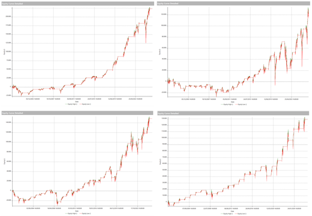
Figure 2 – Equity curves for the buy-and-hold approach and the three seasonal windows.
First Half vs. Second Half: What Does the Backtest Reveal?
Looking at the results shown in Figure 2, we can see that the equity curves for all three seasonal windows are consistent with the patterns identified by Bias Finder. All three generated positive net profits, but performance improved as we moved toward the seasonal windows in the second half of the year. Nearly all metrics improved, particularly maximum drawdown.
In fact, when moving from the first six-month window to the final three-month window, from October through December, the maximum drawdown was reduced by more than half, while the average trade increased by nearly 50%. This result is also reflected in the exceptionally smooth equity curve.
As expected, the Buy and Hold approach outperformed all the other alternatives in terms of net profit because of its significantly longer time in the market. However, it was also exposed to much greater fluctuations, as demonstrated by its maximum drawdown of -$69,337.50. This was identical to the drawdown recorded by the least favorable seasonal window, Window No. 1, covering the first six months of the year.
Table 1 – Performance comparison of the three seasonal windows on E-mini S&P 500 futures (@ES).
| Net Profit | Avg. Trade | Percent Profitable | No. of Trades | Max Drawdown | |
| Buy & Hold | $223,487.50 | $15,963.39 | 71.43% | 14 | -$69,337.50 |
| Seasonal Window 1 – January through June | $94,587.50 | $3,637.98 | 69.23% | 26 | -$69,337.50 |
| Seasonal Window 2 – July through December | $148,787.50 | $5,722.60 | 65.38% | 26 | -$47,587.50 |
| Seasonal Window 3 – October through December | $128,887.50 | $4,957.21 | 88.46% | 26 | -$30,350.00 |
Can Performance in the First Six Months Influence the Rest of the Year?
We will now focus on the two most interesting seasonal windows, Windows No. 2 and No. 3, to determine whether their performance is actually correlated with market performance during the first half of the year.
For Seasonal Windows No. 2 and No. 3, positions will be entered using the same rules described above, but only if E-mini S&P 500 futures (@ES) posted a positive return during the first half of the year.
We will also test different first-half performance thresholds to determine whether any specific level can further improve the strategy’s performance metrics.
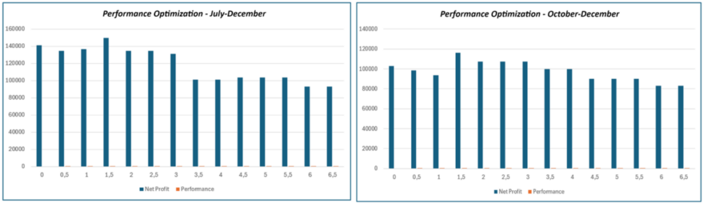
Figure 3 – Optimization of the first-half performance threshold for the July-December window, left, and the October-December window, right.
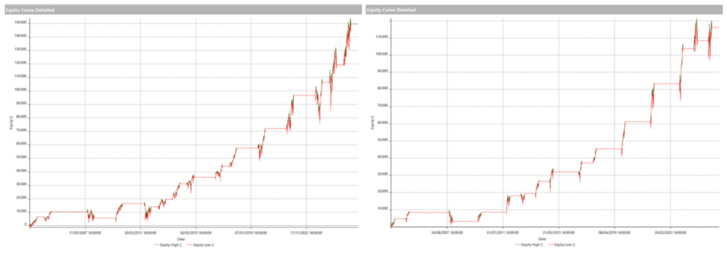
Figure 4 – Equity curve for the July-December window with a first-half performance filter above 1.5%, left, and equity curve for the October-December window with a first-half performance filter above 1.5%, right.
Does the First-Half Performance Filter Improve the Results?
Table 2 shows that applying a filter requiring positive performance during the first six months already produces interesting results. For Seasonal Window No. 2, net profit decreases slightly, but risk is significantly reduced, with maximum drawdown falling from more than $47,000 to approximately $33,000. The average trade rises above $7,000, while the percentage of profitable trades approaches 80%.
The results for Seasonal Window No. 3 are even more pronounced: the percentage of profitable trades approaches 90%, while maximum drawdown declines from approximately $30,000 to just over $25,000.
Table 2 – Results for the seasonal windows on E-mini S&P 500 futures (@ES) after applying the first-half performance filter.
| Net Profit | Avg. Trade | Percent Profitable | No. of Trades | Max Drawdown | |
| Seasonal Window 2 – Performance > 0% | $140,975.00 | $7,831.94 | 77.78% | 18 | -$33,050.00 |
| Seasonal Window 2 – Performance > 1.5% | $149,612.50 | $9,974.17 | 86.67% | 15 | -$30,062.50 |
| Seasonal Window 3 – Performance > 0% | $96,887.50 | $5,382.64 | 88.89% | 18 | -$25,575.00 |
| Seasonal Window 3 – Performance > 1.5% | $108,312.50 | $7,220.83 | 93.33% | 15 | -$21,437.50 |
Raising the performance threshold above zero, and therefore requiring a stronger bullish trend during the first half of the year, maximizes net profit for both seasonal windows at approximately the 1.5% level, as shown in Figure 3. Beyond this threshold, the filter becomes much more selective. As a result, the strategy takes significantly fewer trades, leading to a predictable decline in overall net profit.
What Can We Learn From This Analysis of S&P 500 Seasonality?
In this article, we found that E-mini S&P 500 futures (@ES) exhibit certain patterns throughout the trading year that may not be immediately obvious or predictable. Understanding these dynamics could prove useful both when developing trading systems and when making asset allocation decisions.
We also identified a positive correlation between performance during the first six months of the year and performance throughout the remainder of the year. This characteristic could help traders identify the years offering the most favorable conditions for entering a position.
There may be many different explanations for these seasonal tendencies. One factor that should not be overlooked, however, is investor psychology, which has always played a fundamental role in financial markets.
At this point, I will leave it to you to explore additional seasonal windows. For example, instead of using performance during the first six months as a filter, you could analyze performance over other periods, such as the first nine months of the year, from January through September.
As always, the possibilities are virtually endless. However, when working with strategies of this kind, particular care should be taken before adding further conditions, given the very limited statistical sample of trades.
Until next time, happy trading!
Credit for images: Author
Benzinga Disclaimer: This article is from an unpaid external contributor. It does not represent Benzinga’s reporting and has not been edited for content or accuracy.
Login to comment